Table of Contents
The same resistance temperature detector can produce different temperature errors when connected with two, three or four wires. An interface with more ADC bits will not remove a lead-resistance error that the wiring topology leaves inside the measurement.
When procuring an RTD input module or selecting its analog front end, begin with the sensor type, cable arrangement and allowed temperature error. The interface must support that installation, including its lead resistance, excitation and input-voltage limits.
Which RTD connection is appropriate for the error budget?
A two-wire connection is suitable when lead resistance is small enough or can be acceptably corrected. Three-wire circuits compensate lead resistance under matching assumptions. Four-wire sensing separates the excitation path from the voltage-sensing path and is useful when lead resistance would otherwise consume too much error budget.
TI’s basic guide to RTD measurements presents the different topologies and their operating constraints. A three-wire terminal block alone does not establish the quality of compensation; the current-source arrangement and measurement method matter.
| Connection | Main advantage | Remaining condition to check |
|---|---|---|
| Two-wire | Simple wiring and fewer terminals | Lead resistance appears in the measurement |
| Three-wire | Compensation with one fewer wire than four-wire sensing | Lead and excitation matching assumptions |
| Four-wire | Separate force and sense paths | Input bias, compliance, protection and sensor errors still remain |
Choose the topology from the allowed error and installation constraints, not from an assumption that more wires always improve every aspect of the channel.
How much temperature error can lead resistance create?
Convert the resistance error to a local temperature error using the sensor’s resistance-versus-temperature slope. The slope depends on sensor type and temperature, so a single conversion factor should not be used across an unrestricted range.
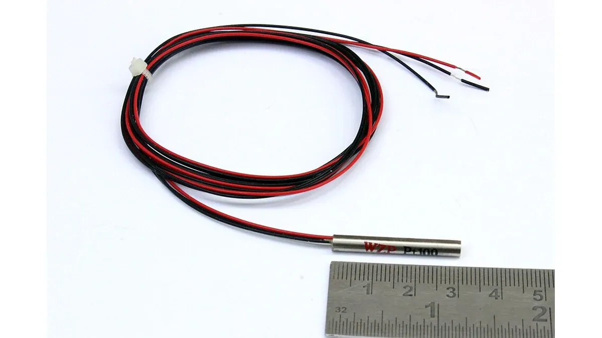
For a standard PT100 near 0°C, the local slope from the usual Callendar–Van Dusen relation is approximately 0.3908 Ω/°C. In a hypothetical two-wire circuit with 1 Ω in each lead, the added 2 Ω corresponds to roughly:
ΔT ≈ 2 / 0.3908 = 5.12°C
That is an illustrative local linearization, not a full-range temperature conversion. Cable resistance also changes with temperature, so a fixed correction can leave a varying residual error.
For a three-wire method whose residual equals a 0.1 Ω lead mismatch, the same local estimate is about 0.26°C. The actual relationship must be derived from the chosen circuit; not every three-wire topology has the same error terms.
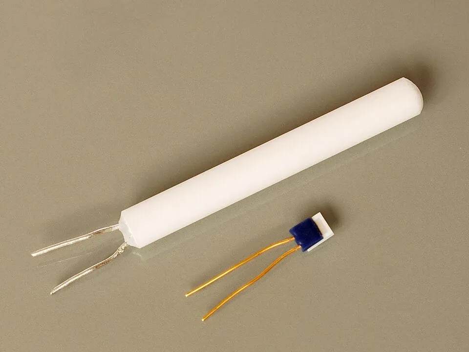
Why can a larger excitation current reduce overall accuracy?
More excitation produces a larger voltage signal, but also increases sensor power and may exceed circuit headroom. The resulting self-heating can offset the benefit of a larger signal.
At 1 mA through a 100 Ω sensor, the dissipated power is 0.1 mW. At 2 mA, it becomes 0.4 mW. Converting that power to a temperature rise requires the sensor’s dissipation characteristics and its installed thermal environment.
A probe in moving liquid can behave differently from the same element in still air or poorly coupled to a surface. Use the sensor manufacturer’s conditions rather than assigning a universal temperature rise per milliamp.
Check the current source’s compliance and the ADC’s common-mode range at the highest sensor and lead resistance. Protection resistors and filters also consume voltage headroom. An interface can be accurate around room temperature yet leave its permitted range near the top of the measurement span.
Build the input specification around independent errors
Separate sensor tolerance, lead effects, reference uncertainty, ADC and amplifier errors, self-heating and temperature conversion. Avoid adding all of them as if they were identical random errors; distinguish bounded limits from statistical uncertainty and from correctable offsets.
Ratiometric measurement can reduce sensitivity to common excitation variation when the sensor and reference share the appropriate current relationship. It does not remove reference-resistor tolerance, mismatch or every temperature effect.
The procurement specification should state the RTD nominal resistance and characteristic, supported wiring modes, excitation range, lead-resistance limit, input range, temperature range, required channel accuracy and test conditions. This is a different task from thermocouple cold-junction compensation.
How should a replacement RTD interface be qualified?
Verify electrical behavior with known resistances and representative lead networks, then test the complete sensor installation where thermal effects matter. Include open and shorted sensor conditions if the application relies on fault reporting.
Exercise the specified temperature endpoints, lead mismatch and channel-switching sequence. Retain the gain, data rate, filter and excitation settings with the results. A successful reading at one resistance does not qualify the full channel.
The final approval should identify both the interface configuration and the supported sensor installation. That prevents an electrically similar replacement from being used with a cable or probe arrangement it was never evaluated to support.
Frequently Asked Questions (FAQ)
Can a PT1000 be substituted for a PT100 without changing the electronics?
Not automatically. The nominal resistance changes by a factor of ten, affecting excitation voltage, gain, reference sizing, input range and the conversion configuration.
Does a four-wire connection remove sensor tolerance?
No. It reduces lead-resistance influence on the voltage measurement. Sensor tolerance, drift, self-heating, reference error and other system errors remain.
Is a resistance simulator enough to qualify a complete temperature channel?
It is useful for evaluating the electrical interface, but does not reproduce sensor self-heating, thermal contact, response time or installation gradients. Include the actual sensor where those effects matter.